Self-Organizing Maps For Machine Learning: A Practical Guide

Self-organizing maps (SOMs), also known as Kohonen maps, are a type of artificial neural network used for unsupervised learning tasks such as cluster neural networks used for unsupervised learning tasks such as clutter and reduced dimensionality. SOMs train using a competitive learning algorithm, in which neurons compete to represent the input data. This results in a two-dimensional grid of neurons, where similar data points map to nearby neurons.

This blog post introduces self-organizing maps (SOMs) and their applications, including fraud detection. Also provides a step-by-step guide to implementing SOMs for fraud detection.

What is a Self-Organizing Map(SOM)?

Imagine you have a map, and you want to organize data points on it in a way that captures their inherent structure and relationships. This is precisely what a Self-Organizing Map (SOM) does in the world of machine learning. SOM was developed by Teuvo Kohonen in the 1980s.

At its core, SOM consists of an array of neurons arranged in a grid-like fashion. Each neuron has an associated weight vector that represents a point in the data space. During training, SOM learns to adapt these weight vectors to the input data in a way that nearby neurons on the map respond to similar input patterns. This self-organization process is what makes SOM so powerful.

How Does SOM Work?

SOM architecture works based on a two-dimensional grid of neurons. Each neuron in the grid has a weight vector that initializes randomly. The weight vector represents the position of the neuron in the input space.

Step-by-step guide to how a SOM works

• Initialization

  Each neuron's weight vector is assigned random values or values drawn from the input data.

• Competition and Cooperation

  When presented with an input data point, neurons compete to be the best match. The winning neuron (the one with the closest weight vector) and its neighbors are updated to become more similar to the input.

• Iterative Learning

  This process is repeated for multiple data points, gradually fine-tuning the neurons' weight vectors.

Over time SOM neurons learn to represent different features of the input data, which organizes the data into a two-dimensional map.

Also Read: How to Use Linear Regression to Make Predictions in Machine Learning

Applications of SOMs

SOMs have a wide range of applications in machine learning, including:

• Data Clustering

  On a map, SOM can be used to cluster similar data points together. This helps identify natural groupings or patterns within complex datasets.

• Dimensionality Reduction

  With SOM, the dimensions of data are reduced while their structure is preserved. Visualizations and feature selections can be made using this method.

• Data Visualization

  A SOM creates 2D and 3D representations of high-dimensional data that make it easier for humans to interpret and comprehend.

• Anomaly Detection

  An anomaly or outlier can be detected using SOM by identifying data points that do not conform to established patterns.

• Customer Segmentation

  In marketing and business, SOM can be applied to segment customers based on their behavior which allows for targeted marketing strategies.

Implementation of Fraud Detection Using SOMs

SOMs can be used to implement a fraud detection system by following these steps:

Part 1: Data Preprocessing

Preprocess the data to ensure that it is in a format that is compatible with the SOM algorithm. To process the data you have to execute the given steps:

1.1 Import Libraries

To execute data processing we have to implement 3 libraries,

• NumPy Library, used for multidimensional array
• Pandas Library, used for importing the dataset
• Matplotlib Library, used for plotting the graph

# import the libraries
import numpy as np
import pandas as pd
import matplotlib.pyplot as plt

1.2 Import Dataset

To import the dataset we use Pandas library to load the Credit Card Application dataset from Kaggle into a DataFrame. then split the dataset into independent and dependent variables using the iloc function, which we store in the variables X and y, respectively.

# import the database from kaggle
dataset = pd.read_csv('Credit_Card_Applications.csv')

#independent variables
X = dataset.iloc[:, :-1].values 

# dependent variables
y = dataset.iloc[:, -1].values 

1.3 Feature Scaling

It is important in data preprocessing because it helps to normalize the features so that they have the same scale. This makes it easier for machine learning algorithms to learn from the data. The MinMaxScaler class from the scikit-learn library is a popular normalization technique that scales the features so that they fall within the range [0, 1].

from sklearn.preprocessing import MinMaxScaler
sc = MinMaxScaler(feature_range = (0,1))
X = sc.fit_transform(X)

Part 2: Train model

Train a SOM on the preprocessed data.

2.1 Import The Model

If you use the MiniSom model for SOMs and you get an error, you need to install it using the following command:

#!pip install minisom
from minisom import MiniSom

2.2 Initialize SOM Model

To initialize a SOM model, we need to specify a few parameters:

• Dimensions of the SOM Map

  This defines the size of the SOM grid. For example, a 10x10 grid would have 100 nodes.

• Input Length

  This is the number of features in the input data. For example, we have 15 different attributes available in the dataset, we take input_length = 15.

• Neighborhood Radius

  This defines the size of the neighborhood around the best matching unit (BMU) that is updated during training. A larger neighborhood radius will result in smoother updates to the SOM weights. Here we’ll use a 1.0 radius.

• Learning Rate

  It is a hyperparameter, that defines how much the SOM weights are updated during each iteration of training which is default is 0.5.

som = MiniSom(x=10,y=10,input_len=15, sigma=1.0,learning_rate=0.5)

2.3 Initialize The Weight

We randomly initialize the weights of our SOM model using our data (X).

som.random_weights_init(X)

2.4 Train the model

In this step, we train the SOM model. We pass two parameters to the training function: the input data and the number of iterations. In this example, we choose 100 iterations.

som.train_random(data = X, num_iteration = 100)

Part 3: Visualize The Model

To simply visualize a self-organizing map(SOM) use the following code:

# Imports the necessary libraries from pylab
from pylab import bone, pcolor, colorbar, plot, show

#Creates a bone colormap.
bone()

#Creates a pcolor plot of the SOM's distance map
pcolor(som.distance_map().T)

#Adds a colorbar to the plot
colorbar()

#Defines the marker types and colors that will be used to plot the data points
markers = ['o','s']
colors = ['r','g']

#Iterates over the input data
for i,x in enumerate(X):

#Finds the winning node for the current data point
w = som.winner(x)

#Plots a marker at the winning node for the current data point
plot(w[0] + 0.5,
      w[1] + 0.5,
      markers[y[i]],
      markeredgecolor = colors[y[i]],
      markerfacecolor = 'None',
      markersize=10,
      markeredgewidth=2)

#Displays the plot
show()

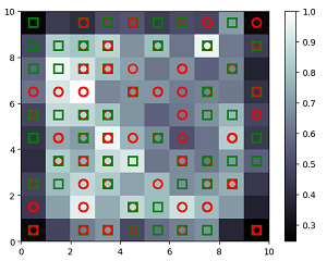
The Self-Organizing Map (SOM) visualizes customer data, where red circles represent customers who did not get approval and green squares represent customers who did get approval. Outliers, shown in white, have a high potential for fraud.

Part 4: Catch the Potential Fraud

4.1 Map the winning node

To catch the potential fraud, we need to map the winning code using the given code.

# mapping the winning node
mappings = som.win_map(X)

The code creates a dictionary that maps each winning node to its customers. This dictionary can be used to identify potential fraud by looking for customers that are mapped to winning nodes with high inter-neuron distances (IND). IND is a measure of how different a winning node is from its neighbors. Outlier data points, such as fraudulent customers, are more likely to have higher INDs.

4.2 Catch The Cheater

Use the given Python code to catch the cheater using SOM.

frauds=np.concatenate((mappings[(7,8)], mappings[(3,1)], mappings[(5,1)]), axis=0)

The code first uses a self-organizing map (SOM) to map the winning node for each customer. The winning node is the node on the SOM that is most similar to the customer's data. The code then takes only the customers whose winning nodes are [(7,8), (3,1), and (5,1)]. These customers are flagged as potential fraud customers because their winning nodes are outliers on the SOM.

4.3 Rescale the value

# Rescale the values of the potential fraud customers
for i in range(len(frauds)):
    frauds[i] = inverse_scale_function(frauds[i])

This code will rescale the values of the potential fraud customers back to the original scale using the inverse scale function. The inverse scale function scales the values before training the SOM.

Part 5: Final Result

# Print the list of potential fraud customers in the original scale
print(frauds)

The final result of catching fraud using SOM is a list of customers who are most likely to be cheating. The generated list by SOM helps to identify customers whose winning nodes are outliners. The winning node for a customer is the node on the SOM that is most similar to the customer's data.

Conclusion

The guide will help you to find fraud detections using SOMs. Also, Self-Organizing Maps (SOMs) are a powerful type of unsupervised machine-learning algorithm that helps to reduce dimensionality, visualize data, and cluster data points. It is particularly useful for analyzing high-dimensional data, as it can project the data into a lower-dimensional space while preserving the underlying relationships between the data points.

If you are working with high-dimensional data or if you need to develop a machine learning algorithm that can learn without labeled data, then SOMs are a good option to consider.

Get a free consultation for AI & ML from CodeTrade, a leading AI & ML Development Company in India. We offer a free consultation to help you understand how to use AI and ML to improve your business. Our team of experienced AI and ML developers can provide you with high-quality AI and ML services tailored to your specific needs.