Understand the Grad-CAM: A Complete Guide With Example

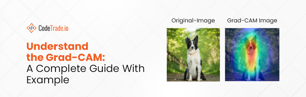
Gradient-weighted Class Activation Mapping (Grad-CAM) is a technique in deep learning and computer vision that helps to visualize the areas of an image that a convolutional neural network (CNN) focuses on when making predictions. It is a powerful tool for understanding what parts of an image are most important in the decision-making process of a neural network.

In this blog, we'll walk through the Grad-CAM process step by step and provide Python code to demonstrate how to generate Grad-CAM heatmaps and determine the steps to apply Grad-CAM in Deep Learning. We'll use a pre-trained model and a sample image for illustration.

Concept of Grad-CAM

One of the popular techniques for visualizing the Convolutional Neural Network Model is Gradient-Weighted Class Activation Mapping(Grad-CAM). Grad-CAM is class-specific and produces a separate visualization for each image input class.

In the world of deep learning, especially with convolutional neural networks (CNNs), Grad-CAM helps to understand the parts of an image that CNN focuses on when making a specific prediction.

Unlike other visualization methods, Grad-CAM keeps the original structure of the deep learning model intact and provides clear explanations without needing to rebuild or retrain it. Grad-CAM can pinpoint image regions crucial for a particular class while generating high-resolution visualizations for better understanding. Before we dive into the details of how Grad-CAM works, let's briefly review the steps involved in the Grad-CAM process:

Grad-CAM Process Overview

We will break down the Grad-CAM process into the following steps:

• Load and Preprocess the Image: Load an image from a URL, resize it to a size compatible with our model, and preprocess it.

• Create Grad-CAM Model: Create a modified model that takes the original model's inputs and outputs from the desired convolutional layer and the final prediction.

• Calculate Gradients: Calculate the gradients of the predicted class score with respect to the feature maps of the chosen convolutional layer.

• Generate the Heatmap: Using the gradients, we can calculate the weighted combination of feature maps to create the Grad-CAM heatmap.

• Display Heatmap: Overlay the heatmap on the original image to visualize which parts of the image are critical for the model's decision.

Prerequisites

Before we begin working with the code, must ensure that you have the required libraries installed.

1. TensorFlow (for deep learning operations)
2. NumPy (for numerical operations)
3. PIL (Python Imaging Library, for image processing)
4. Matplotlib (Used for visualize images and heatmaps)
5. Requests (Used for download images from URLs)

You can use the following command to install these Python libraries using pip:

pip install tensorflow numpy pillow matplotlib requests

Let’s explore the step-by-step process to apply Grad-CAM to Deep Learning Models.

Steps to Apply Grad-CAM to Deep-Learning Models

Follow the given steps to Apply Grad-CAM to Deep-Learning Models:

Step 1: Load and Preprocess the Image

In the first step, we need to load and prepare the image for the process. Create a function called get_processed_img that performs the following tasks:

• Downloads an image from a URL.
• Resize the image to a standard input size (224x224 pixels).
• Preprocesses the image by normalizing pixel values to the range [0, 1].

Use the given code for this step:

import PIL
import numpy as np
import requests

def get_processed_img(url):
    # Open the image using the URL
    img_from_url = PIL.Image.open(requests.get(url, stream=True).raw)
    
    # Adjust the image dimensions to a standard size.
    new_image = img_from_url.resize((224, 224))
    
    # Transform the image into a NumPy array.
    processed_image = np.asarray(new_image)
    
    # Normalise pixel values if necessary
    if processed_image.max() > 1:
        processed_image = processed_image / 255
    
    # Add a batch dimension
    image = np.expand_dims(processed_image, axis=0)
    
    return image

Step 2: Create the Grad-CAM Model

In this step, we create a modified model that can generate Grad-CAM heatmaps. This revised model takes the original model's inputs and two outputs: the output of the desired convolutional layer and the final prediction. We use TensorFlow to define this model. For example,

import tensorflow as tf

def make_gradcam_heatmap(img_array, model, last_conv_layer_name, pred_index=None):
    # Create a sub-model that outputs the feature maps and final prediction
    grad_model = tf.keras.models.Model(
        [model.inputs], [model.get_layer(last_conv_layer_name).output, model.output]
    )

    # Use GradientTape to record gradients
    with tf.GradientTape() as tape:
        last_conv_layer_output, preds = grad_model(img_array)
        
        # If pred_index is not specified, use the predicted class index
        if pred_index is None:
            pred_index = tf.argmax(preds[0])
        class_channel = preds[:, pred_index]

    # Calculate gradients
    grads = tape.gradient(class_channel, last_conv_layer_output)
    pooled_grads = tf.reduce_mean(grads, axis=(0, 1, 2))

    # Compute the heatmap
    last_conv_layer_output = last_conv_layer_output[0]
    heatmap = last_conv_layer_output @ pooled_grads[..., tf.newaxis]
    heatmap = tf.squeeze(heatmap)

    # Normalise the heatmap
    heatmap = tf.maximum(heatmap, 0) / tf.math.reduce_max(heatmap)
    
    return heatmap.numpy()

Step 3: Calculate Gradients

Using TensorFlow's GradientTape to calculate the gradients of the predicted class score with respect to the feature maps of the chosen convolutional layer. These gradients will be used to generate the heatmap. To calculate gradients in Grad-CAM, you can use the following steps:

1. Feed the input image to the trained model.
2. Calculate the result of the final convolutional layer.
3. Compute the gradient of the output of the last convolutional layer with respect to the target concept.
4. Take a global average pooling of the gradient map.

Step 4: Generate Heatmap

With the gradients in hand, we combine them with the feature maps of the chosen layer to create the Grad-CAM heatmap. The heatmap highlights the regions of the image that are most influential in making a particular prediction. Normalize the heatmap values to be between 0 and 1.

To generate a Grad-CAM heatmap, follow these steps:

• Multiply the importance weights by the activations of the last convolutional layer.
• Sum the products over the channel dimension.
• Normalize the heatmap.

The heatmap output will highlight the regions of the image that are most important for predicting the target concept.

Step 5: Display Heatmap

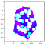
To visualize the results, we define a function called display_gradcam. This function takes the original image, the Grad-CAM heatmap, and an optional alpha value to control the heatmap's transparency. It overlays the heatmap on the original image and displays the result. You can use the given code to display the heatmap in Grad-CAM.

import matplotlib.pyplot as plt
from matplotlib import cm

def display_gradcam(img, heatmap, alpha=0.4):
    # Rescale heatmap to a range of 0-255
    heatmap = np.uint8(255 * heatmap)
    
    # Use the "jet" colormap to colourize the heatmap
    jet = cm.get_cmap("jet")
    jet_colors = jet(np.arange(256))[:, :3]
    jet_heatmap = jet_colors[heatmap]
    
    # Transform the heatmap into an image.
    jet_heatmap = tf.keras.utils.array_to_img(jet_heatmap)
    
    # Resize the heatmap to match the image dimensions
    jet_heatmap = jet_heatmap.resize((img.shape[2], img.shape[1]))
    jet_heatmap = tf.keras.utils.img_to_array(jet_heatmap)
    
    # Superimpose the heatmap on the original image
    superimposed_img = jet_heatmap * alpha + img
    plt.imshow(superimposed_img[0])

You used the following code to generate the given result:

densenet_model = DenseNet201(include_top=False, input_shape=(224,224,3))

for layer in densenet_model.layers:
  layer.trainable = False

Flattened_layer = layers.Flatten()(densenet_model.output)
output_layer = layers.Dense(10, activation='softmax')(Flattened_layer)

final_model = tf.keras.models.Model(inputs=densenet_model.input, outputs=output_layer)

Once the model has been trained, use it to generate Grad-CAM heatmaps of images. Here is an example of a heatmap generated for the following image:

img_arr = get_processed_img('https://t3.ftcdn.net/jpg/01/05/57/38/360_F_105573812_cvD4P5jo6tMPhZULX324qUYFbNpXlisD.jpg')

heatmap = make_gradcam_heatmap(img_arr, final_model, 'conv3_block8_2_conv')

plt.axis('off')
plt.matshow(heatmap)
plt.show()

Display Grad-CAM:

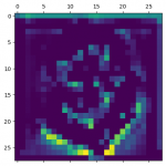
display_gradcam(get_processed_img('https://t3.ftcdn.net/jpg/01/05/57/38/360_F_105573812_cvD4P5jo6tMPhZULX324qUYFbNpXlisD.jpg'), heatmap)

Grad-CAM can be used to interpret the predictions of any deep-learning model that outputs a class probability distribution. It is a powerful tool for understanding how deep-learning models make decisions.

Limitations and Challenges of Grad-CAM

Grad-CAM, while a helpful technique for visualizing what a CNN focuses on in an image, has its limitations and challenges. Here are some of the key limitations to be aware of:

• Localization Accuracy

  Localization can be rough, especially for intricate objects or small details. For that reason, Grad-CAM might not perfectly pinpoint the most relevant parts of an image. This is because it relies on gradients, which can be noisy and not properly aligned with the true importance of a region.

• Multiple Objects of the Same Class

  If an image contains multiple instances of the same predicted class, Grad-CAM may struggle to differentiate between them. The heatmap might highlight areas from all the objects instead of isolating the specific one influencing the prediction.

• Interpretability vs. Accuracy Trade-off

  Complex models that are highly accurate may not be as interpretable with Grad-CAM. This is because it can be difficult to capture the inner workings of such models through Grad-CAM's visualization. It is important to strike a balance between achieving high accuracy and understanding how the model arrives at its decisions.

• Computational Overhead

  Generating Grad-CAM heatmaps can be computationally demanding, especially for very large datasets or complex models. This can be a hurdle for real-time applications or scenarios requiring quick analysis of large amounts of data.

• Network Architecture Limitations

  The standard Grad-CAM formulation works best with CNNs that have Global Average Pooling (GAP) before the final layer. Networks without GAP might require alternative methods like Guided Grad-CAM, which can introduce additional complexities.

• Limited to Convolutional Neural Networks (CNNs)

  Grad-CAM is primarily designed for CNN-based architectures. It relies on the gradients of the target class score for the feature maps, which are specific to CNNs. It may not be directly applicable to other types of neural networks like recurrent neural networks (RNNs) or transformer-based architectures.

Use cases of Grad-CAM

Grad-CAM (Gradient-weighted Class Activation Mapping) is used to understand how deep learning models, particularly Convolutional Neural Networks (CNNs), arrive at their decisions for image classification tasks. Here are some common use cases for Grad-CAM:

1. Understanding Model Decisions

Grad-CAM helps visualize which parts of an image are most important to a model's prediction. This is useful for generally understanding how a CNN reasons and where it focuses its attention.

2. Identify mistakes and Improve Models

If a model makes mistakes or exhibits biases, Grad-CAM can help identify the root cause. By seeing which regions the model focuses on for incorrect predictions, developers can diagnose issues and improve the model's architecture or training data.

3. Biomedical Image Analysis

In medical imaging (X-rays, MRIs), Grad-CAM can highlight areas of interest like tumors or abnormalities. This can assist doctors in diagnosis, treatment planning, and understanding where the model is focusing its attention.

4. Fine-tuning Transfer Learning

Grad-CAM helps fine-tune pre-trained models by revealing important image regions for new tasks, reducing bias, and improving focus.

5. Visual Language Tasks

Grad-CAM explains predictions in visual question answering and image captioning by highlighting relevant image areas and building trust in their reasoning.

Conclusion

In this comprehensive guide, we have explored the powerful concept of Gradient-weighted Class Activation Mapping (Grad-CAM) in the context of machine learning and computer vision. Grad-CAM is an invaluable tool that allows us to visualize and interpret the inner workings of deep learning models, shedding light on the specific regions of an image that influence their predictions.

By following these steps and running the provided Python code, you can easily apply Grad-CAM to your deep-learning models and gain valuable insights into their decision-making processes.

In the ever-evolving field of machine learning and computer vision, techniques like Grad-CAM play a crucial role in making AI systems more transparent, interpretable, and accountable. As you continue your journey in this exciting field, consider incorporating Grad-CAM into your toolbox for model interpretation and transparency.

If you need professional help with your AI/ML project, contact CodeTrade India, a leading AI/ML development company. Our experienced AI/ML developers can help you take your project to the next level. Contact us today for a free consultation.